course: (ML Series) Introduction to Machine Learning III
By Julien Hernandez Lallement, 2021-03-02, in category Course
By Julien Hernandez Lallement, 2021-03-02, in category Course
This post is the third and last part, that followsthe first and second post on introdution to Machine Learning.
It comes a bit late after the first two posts...I got a bit lost in other projects.
I use several materials to prepare this, such as lectures I attended back in Amsterdam and different books, such as this one and that one. Some of this content is inspired (in some cases, directly copied) from other notebooks acquired during Data Science courses I attended in Amsterdam. I unfortunately do not know the authors, so I cannot reference them. Thanks to these anonymous benefactors :)
Here, I will:
The performance metric should be chosen basedon the business case at hand:
I already talked about the mean squared error metric in the first post introducing Machine Learning. Let's review it, and mention other possible metrics used in regression problems.
Mean squared error (MSE): loss function
$$MSE=\frac{1}{N}\sum_{i=1}^N\left(y_i-\hat{y}_i\right)^2$$Regression algorithms use by default an $R^2$ scoring method, the so-called explained variance score or coefficient of determination, calculated as
$$ R^2 = 1 - \frac{\mathrm{residual \, sum \,of \, squares}}{\mathrm{total \,sum \, of \, squares}} = 1 - \frac{ \lvert \lvert \mathrm{\mathbf{y_{test}}} - \mathrm{\mathbf{y_{pred}}} \rvert \rvert^2}{ \lvert \lvert \mathrm{\mathbf{y_{test}}} - \overline{\mathrm{\mathbf{y_{test}}}} \rvert \rvert^2} $$whose highest score, attained after a perfect prediction, is 1. The figure below will help us to wrap our heads around what it is we're trying to calculate, where $f$ in the right figure corresponds to $y_{pred}$:
 Source: https://commons.wikimedia.org/w/index.php?curid=11398293
The image on the left is the square of the distance from the test values to the average true value, while the image on the right is the square of the distance from the test values to the predicted values. The fraction is therefore the sum of the areas of the blue squares divided by the sum of the red squares, or a comparison of our prediction to a random guess. To minimize this fraction (and thus maximize the $R^2$ score), the goal is thus to minimize the size of the blue squares, i.e. predict a line which comes as close to the true values as possible.
Alternatively, $R^2$ can also be viewed as a normalized version of the MSE: $$R^2 = 1 - \frac{MSE}{Var(y)}$$
Compare the performance of the mean_absolute_error and median_absolute_error on y and y_pred values below and visualize both metrices and the absolute prediction errors:
from sklearn.metrics import mean_absolute_error, median_absolute_error
import numpy as np

y = np.array([0.5, 1.9, 3.5, 1, 6.2, 6.9])
y_pred= np.array([1, 2.1, 3.4 ,3.9 , 6, 7.2])
n = len(y)

mean_error = mean_absolute_error(y, y_pred)
median_error = median_absolute_error(y, y_pred)
print('Mean absolute error: {:1.2f}'.format(mean_error))
print('Median absolute error: {:1.2f}'.format(median_error))
import matplotlib.pyplot as plt
fig,ax = plt.subplots(figsize=(6,4))
fig.set_size_inches(11.0, 8.5)
ax.plot(range(n), np.abs(y-y_pred), label='abs error')
ax.plot([0, n-1], [mean_error]*2, '--', label='mean')
ax.plot([0, n-1], [median_error]*2, '--', label='median')
_ = ax.legend()

Accuracy: fraction of labels that are correctly classified
$$A =\frac{TP + TN}{FP + FN + TP + TN}$$Precision: fraction of positive predictions that are correct
$$P = \frac{TP}{FP + TP}$$Recall: fraction of positive labels that are correctly classified
$$R = \frac{TP}{TP + FN}$$Based on your business case, you might want to optimize the model for a given metric rather than another. For example, say you write a model to detect the likelihood customer have to use a voucher. In that case, it is more important to detect most of the positive cases, while accepting false positive. This is because offering a voucher to someone that won't buy anyway might not be very deleterious for your business, while missing on those that would have bought, would cause your business to loose money. In such cases, optimizing for the precision rathr than accuracy makes more sense.
Below, we use the predicted labels to compute the recall, precision, accuracy and f1-score
from sklearn import metrics

y_true = np.array([1, 0, 0, 0, 1, 0, 1])
y_preds = [[1, 0, 0, 0, 0, 0, 0], [1, 1, 1, 1, 1, 1, 1]]

for y_pred in y_preds:
    print(f'For the predictions: {y_pred}')
    recall = metrics.recall_score(y_true, y_pred)
    precision = metrics.precision_score(y_true, y_pred)
    acc = metrics.accuracy_score(y_true, y_pred)
    f1 = metrics.f1_score(y_true, y_pred)
    print("Recall: {:1.2f}".format(recall))
    print("Precision: {:1.2f}".format(precision))
    print("Accuracy score: {:1.2f}".format(acc))
    print("f1 score: {:1.2f}".format(f1))
    print()
An overview of the common scorers and their related metric functions:
| Scoring | Function |
|---|---|
| Classification | |
| ‘accuracy’ | metrics.accuracy_score |
| ‘average_precision’ | metrics.average_precision_score |
| ‘f1’ | metrics.f1_score |
| ‘f1_micro’ | metrics.f1_score |
| ‘f1_macro’ | metrics.f1_score |
| ‘f1_weighted’ | metrics.f1_score |
| ‘f1_samples’ | metrics.f1_score |
| ‘log_loss’ | metrics.log_loss |
| ‘precision’ etc. | metrics.precision_score |
| ‘recall’ etc. | metrics.recall_score |
| ‘roc_auc’ | metrics.roc_auc_score |
| Scoring | Function |
|---|---|
| Clustering | |
| ‘adjusted_rand_score’ | metrics.adjusted_rand_score |
| Regression | |
| ‘mean_absolute_error’ | metrics.mean_absolute_error |
| ‘mean_squared_error’ | metrics.mean_squared_error |
| ‘median_absolute_error’ | metrics.median_absolute_error |
| ‘r2’ | metrics.r2_score |
A typical workflow of the data treatment part of an project could be depicted as below:
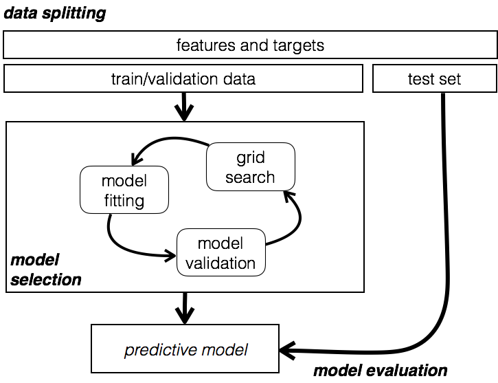
One should not test model performance on data used for training, because we must validate that the model works on unseen data. Training on the whole dataset essentially means we stay in the same place we were before without a way to test how well we do with never before seen data.
The solution is to split the data into different data sets:

In SciKit Learn, the model_selection.train_test_split allows to split data in train/test sets (but easily done without SciKit Learn as well).
Below, a split dividing 40% of the data for the test set.
import pandas as pd
from sklearn.model_selection import train_test_split
from sklearn.datasets import load_boston
from sklearn.preprocessing import StandardScaler

data = load_boston()
X_boston = pd.DataFrame(data.data, columns=data.feature_names)
y_boston = pd.Series(data.target)

# Already scale for future model fit
scaler = StandardScaler()
scaler.fit(X_boston)
scaled_X_boston = scaler.transform(X_boston)

X_train, X_test, y_train, y_test = train_test_split(scaled_X, y, test_size=0.4,
                                                    random_state=42)

print("X shape: {}, y shape: {}".format(
    X.shape, y.shape))
print("X_train shape: {}, y_train shape: {}".format(
    X_train.shape, y_train.shape))
print("X_test shape: {}, y_test shape: {}".format(
    X_test.shape, y_test.shape))
We can then train and test a simple model:
from sklearn.linear_model import SGDRegressor
from sklearn.metrics import mean_squared_error

linear_regression_model = SGDRegressor(tol=.0001, eta0=.01)
linear_regression_model.fit(X_train, y_train)
train_predictions = linear_regression_model.predict(X_train)
test_predictions = linear_regression_model.predict(X_test)

train_mse = mean_squared_error(y_train, train_predictions)
test_mse = mean_squared_error(y_test, test_predictions)

print("Train MSE: {}".format(train_mse))
print("Test MSE: {}".format(test_mse))
Both scores in the train and test sets are quite close, which suggest we are not overfitting. We can look at a learning curve (which plots an error function, in this case MSE, against various amounts of data used for training).
from sklearn.model_selection import learning_curve
from sklearn.metrics import make_scorer
from sklearn.metrics import mean_squared_error
import numpy as np
import matplotlib.pyplot as plt

## source: http://scikit-learn.org/0.15/auto_examples/plot_learning_curve.html
def plot_learning_curve(estimator, title, X, y, ylim=None, cv=None,
                        n_jobs=1, train_sizes=np.linspace(.1, 1.0, 5)):
    """
    Generate a simple plot of the test and traning learning curve.

    Parameters
    ----------
    estimator : object type that implements the "fit" and "predict" methods
        An object of that type which is cloned for each validation.

    title : string
        Title for the chart.

    X : array-like, shape (n_samples, n_features)
        Training vector, where n_samples is the number of samples and
        n_features is the number of features.

    y : array-like, shape (n_samples) or (n_samples, n_features), optional
        Target relative to X for classification or regression;
        None for unsupervised learning.

    ylim : tuple, shape (ymin, ymax), optional
        Defines minimum and maximum yvalues plotted.

    cv : integer, cross-validation generator, optional
        If an integer is passed, it is the number of folds (defaults to 3).
        Specific cross-validation objects can be passed, see
        sklearn.cross_validation module for the list of possible objects

    n_jobs : integer, optional
        Number of jobs to run in parallel (default 1).
    """
    plt.figure()
    plt.title(title)
    if ylim is not None:
        plt.ylim(*ylim)
    plt.xlabel("Training examples")
    plt.ylabel("Score")
    train_sizes, train_scores, test_scores = learning_curve(
        estimator, X, y, cv=cv, n_jobs=n_jobs, train_sizes=train_sizes, scoring=make_scorer(mean_squared_error))
    train_scores_mean = np.mean(train_scores, axis=1)
    train_scores_std = np.std(train_scores, axis=1)
    test_scores_mean = np.mean(test_scores, axis=1)
    test_scores_std = np.std(test_scores, axis=1)
    plt.grid()

    plt.fill_between(train_sizes, train_scores_mean - train_scores_std,
                     train_scores_mean + train_scores_std, alpha=0.1,
                     color="r")
    plt.fill_between(train_sizes, test_scores_mean - test_scores_std,
                     test_scores_mean + test_scores_std, alpha=0.1, color="g")
    plt.plot(train_sizes, train_scores_mean, 'o-', color="r",
             label="Training score")
    plt.plot(train_sizes, test_scores_mean, 'o-', color="g",
             label="Cross-validation score")

    plt.legend(loc="best")
    return plt

plot_learning_curve(linear_regression_model, "Learning Curve", X_train, y_train, cv=5)

We see that with less than ~80 training examples, the score is relatively good on the training set, while the cross-validation is quite high (see below for cross validation). This situation is typical of high variance contexts. However, as we increase our data, we begin to improve both of our scores and they become very close, which suggests we don't have a high variance problem.
In the plot above, you see that the green line corresponds to cross validation. What does that mean?
While the approach of splitting data into train/test sets is the basics, simple dataset splitting as done above is often problematic, becacuse (i) we want to learn from as much data as possible and (ii) we also want to test on a large data set, which reduces the size of the training set in case of single splits.
One can then use third a set of data - a validation set. Basically, what we can do is break down our training data into two sets: a training set and a validation set. All models will be trained on the training set and then tested on our validation set. We then take the model that does the best on validation and see how well it does on testing. Our testing results represent how well we think our model would do with unseen data - and then we are done. One important assumption here though is that the train set and validation set are representative of the population from which the data is drawn.
In practice, instead of creating one single validation set, we create a number k of them. So called K-fold cross-validation do this for us and splits the data into $k$ independent folds. One can then (i) fit the model on $k−1$ train folds, (ii) estimate performance on the remaining fold and (iii) repeat this procedure $k$ times.
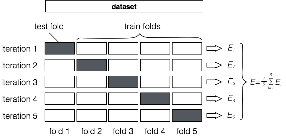
This approach is quite powerful, since it allows us to repeatedly evaluate our model. Below, we compute the accuracy of a Logistic Regression using cv = 5 Folds cross validation
from sklearn.model_selection import cross_val_score
from sklearn.linear_model import LogisticRegression
from sklearn.metrics import f1_score
from sklearn.datasets import load_iris

data = load_iris()
X = pd.DataFrame(data.data, columns=data.feature_names)
y = pd.Series(data.target)

scaler = StandardScaler()
scaler.fit(X)
scaled_X = scaler.transform(X)

clf = LogisticRegression(C=0.1)

scores = cross_val_score(clf, scaled_X, y, cv=5, scoring='accuracy')

print("Scores per fold: {}".format(scores))
print("Mean accuracy: {0:.2f}".format(scores.mean()))
You can play around with different parameters of K fold cross validation here to understand a bit better what's happening under the hood.
While the number of folds in cross validation is the most basic parameter, we can edit additional parameters such as the type of cross validation we want to perform (StratifiedKFold, ShuffleSplit, LeavePOut). I won't be going into details about this topic in this introduction.
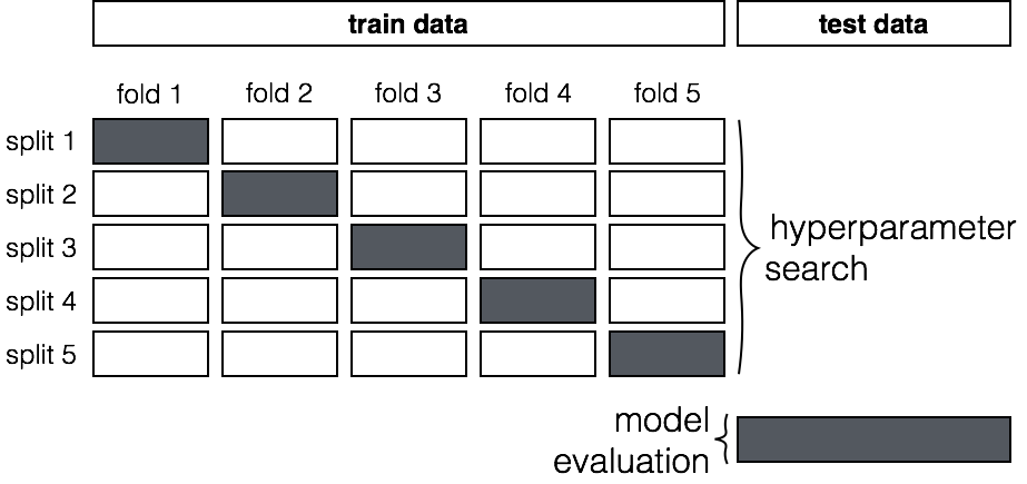
Model hyperparameters teach the model how to learn. These are number and depth of trees in RandomForest algorithms, or regularization strength in LASSO & Ridge regressions.
The most famous way to tune these hyperparameters (to obtain a better model fit) is GridSearch. This approach is a quite crude technique to test over a set of possible hyperparameters, typically dictated by the user based on experience & common sense.
One would:
Using the same boston dataset as before:
X_train, X_test, y_train, y_test = train_test_split(scaled_X_boston, y_boston, test_size=0.33, random_state=42)
from sklearn.model_selection import RandomizedSearchCV

param_dist = {"eta0": [ .001, .003, .01, .03, .1, .3, 1, 3],
             "tol": [0.01, 0.001, 0.0001]}

linear_regression_model = SGDRegressor()

n_iter_search = 8
random_search = RandomizedSearchCV(linear_regression_model, param_distributions=param_dist,
                                   n_iter=n_iter_search, cv=3, scoring='neg_mean_squared_error')
random_search.fit(X_train, y_train)

print("Best Parameters: {}".format(random_search.best_params_))
print("Best Negative MSE: {}".format(random_search.best_score_))
As you can see, I used Randomized search instead of GridSearch, which typically is better than searching over all possible values. Often, you want to try many different parameters for many different knobs and grid searching over everything is not efficient. Given the small number of iterations, GridSearch would have worked as well, but now you've heard of this approach as well ;)
If you got up to here, then here is al little bonus ;)
Once you obtain your trained model, you should not do as I most of the time do (bad Julien...): retrain everytime. It takes time, it's bad for the environment, and it simply stupid (doing every time the same thing).
There are two methods you can use to store trained models for future use:
pickle: using Python’s built-in persistence model; can pickle to both disk and stringjoblib: similar to pickle only more efficient on objects that carry large numpy arrays; can only pickle to disk# use joblib to store on disk
from sklearn import datasets
from sklearn import svm
import joblib
! mkdir '../output'
clf = svm.SVC()
data = load_iris()
X = pd.DataFrame(data.data, columns=data.feature_names)
y = pd.Series(data.target)
clf.fit(X, y)
joblib.dump(clf, filename='../output/iris_svc.pkl')
clf_j = joblib.load(filename='../output/iris_svc.pkl')
print("prediction with reloaded clf: {}".format(clf_j.predict(X.iloc[[0]])))
To rebuild a similar model with future versions of scikit-learn, all metadata should be saved along the pickled model:
